By Sebastian Proft (sebastian.proft AT charite.de)
As the new backbone model for MutationTaster2021, we decided to use a Random Forest model. Random Forests have the useful property of not making assumptions about the distribution of the input data. They also have the advantage of being relatively simple and easy to understand and explain. So, for clarities sake. We will go explain here how they function in detail.
In order to understand how a Random Forest model is built and trained we will first talk about the underlying structure of which it is comprised, which is to say a Decision Tree.
Decision Trees are relatively simple models on which a computer can learn to make decisions based on previously observed information. Let’s take an example:
Let’s say you want to decide whether to cross the street or not. There can be a lot of factors that influence your decision, all based on past experiences. First you could check whether the traffic light is green and you know that every time the traffic light has been green in the past you crossed the street. Very simple. The decision becomes light(green) -> cross(yes). But what happens if the light is red? You know you almost never crossed the street when the light was red, but sometimes you did. What influenced your decision? You might check if a car is coming. And if it is, you do not want to be run over. So, you decide to not cross the street. It becomes light(red) ‑> car(yes) ‑> cross(no). If you realize that there is no car coming, you could finally check if a child is present. Because you for sure do not want to set a bad example. You decide not to cross: light(red) ‑> car(no) ‑> child(yes) ‑> cross(no). If there is no child that you could badly influence, you decide you can cross, albeit quickly: light(red) ‑> car(no) ‑> child(no) ‑> cross(yes).
We have now created a simple decision tree:

What we now have done is walking through every step of constructing the Decision Tree, i.e., we “trained” the model. Of course, what we want is an algorithm, that does the training for us so that we can lean back, relax and enjoy a cocktail (the relaxing is essential for good work and not just because we are lazy).
What we also want to ensure is that our decision tree is at least somewhat efficient in its decisions. Let’s have a look at this tree based on our first example:

This tree comes to exactly the same decisions as the previous tree. You can confirm for yourself if you want. What should be intuitively apparent is that the left car decision is superfluous (i.e., it doesn’t matter whether car is coming, because we are stopping regardless).
So, how does the training work? We usually start from a dataset that includes the outcome (i.e., will we cross the street) for a set of inputs (i.e., is a child present?). We will refer to the outcome as label and the inputs as feature.
Let’s take this input as an example:
| Toothed | Hair | Breathes | Legs | Species |
|---|---|---|---|---|
| Yes | Yes | Yes | Yes | Mammal |
| Yes | Yes | Yes | Yes | Mammal |
| Yes | No | Yes | No | Reptile |
| No | Yes | Yes | Yes | Mammal |
| Yes | Yes | Yes | Yes | Mammal |
| Yes | Yes | Yes | Yes | Mammal |
| Yes | No | No | No | Reptile |
| Yes | No | Yes | No | Reptile |
| Yes | No | Yes | Yes | Mammal |
| No | No | Yes | Yes | Reptile |
We will now walk step by step through this example to construct a fitting decision tree using the CART (Classification And Regression Tree) algorithm, the same one as was used for MutationTaster. CART follows a few simple steps:
Let’s first select our metric. For MutationTaster we used the metrics Entropy and Gini index.
The Gini index scales from 0 to 1, where 0 is a pure class (i.e., all datapoints share the same label) and 1 is an impure class (i.e., we have a 50/50 split in the labels). Here, we will explain how the Gini Index is calculated.
In order to find the best split you have to calculate the Gini index for each of the possible splits. Therefore,
we first pick a potential split let’s say “Toothed”. For “Toothed” we first calculate the probability of its
values:
P(Toothed=Yes) = 8/10
P(Toothed=No) = 2/10
Now we need to calculate the dependent probability of observing our outcome given the observation:
P(Species=Mammal if Toothed=Yes) = 5/8
P(Species=Reptile if Toothed=Yes) = 3/8
And the same for toothed=No:
P(Species=Mammal if Toothed=No)
= 1/2
P(Species=Reptile if Toothed=No) =
1/2
Now we can calculate the Gini index for each branch of the decision tree:
Gini Index (Toothed=Yes) = 1 — {(5/8)² + (3/8)²} = 1 –
0.39 – 0.14 = 0.47
Gini Index (Toothed=No) = 1 — {(1/2)² + (1/2)²} = 1 – 0.25
- 0.25 = 0.5
In order to calculate the best feature to split on we need to calculate the Gini index for this feature. This is
calculated as the weighted average of both Gini indices:
Gini Index (Toothed) = (8/10) * 0.47 + (2/10) * 0.5 = 0.38 + 0.1 = 0.48
This procedure is repeated for each feature:
Gini Index (Hair) = (5/10) * 0 + (5/10) * 0.32 = 0.16
Gini Index (Breathes) = (9/10) * 0.44 + (1/10) * 0 = 0.40
Gini Index (Legs) = (7/10) * 0.25 + (3/10) * 0 = 0.18
As an exercise you can convince yourself that these calculations are correct. So now we know which feature gives us the “purest” splits. It is Hair, because it gives us the lowest Gini index. Now we have the first split for our tree:

We can now split the remaining data and remove Hair as a feature:
| Toothed | Hair | Breathes | Legs | Species |
|---|---|---|---|---|
| Yes | Yes | Yes | Yes | Mammal |
| Yes | Yes | Yes | Yes | Mammal |
| No | Yes | Yes | Yes | Mammal |
| Yes | Yes | Yes | Yes | Mammal |
| Yes | Yes | Yes | Yes | Mammal |
| Toothed | Hair | Breathes | Legs | Species |
|---|---|---|---|---|
| Yes | No | Yes | No | Reptile |
| Yes | No | No | No | Reptile |
| Yes | No | Yes | No | Reptile |
| Yes | No | Yes | Yes | Mammal |
| No | No | Yes | Yes | Reptile |
It is easy to see that we already have a completely pure node. So, after we know that an animal has “Hair” we also know that it has to be a Mammal and we can update our tree accordingly:

This entire process can now be repeated for the case of the animal not having hair. What you will end up with is this tree:

Congratulations with this we have trained a decision tree.
If we want to make a prediction, we get a set of inputs and then go through the tree step by
step.
Does the animal have hair? No
Does the animal have legs? Yes
Does it have teeth? No
Well then, we must be talking about a Reptile.
In some cases, a single Decision Tree might not be enough to truly grasp all the nuances of the training data. Decision Trees also suffer from tending to overfit and, because the CART algorithm decides on splits in a greedy fashion (meaning first come first served), if a feature looks good as the very first split, but could create a better split if used later, it will never be found. A solution to this problem is the power of many. If one decision tree is not good enough. How about we use a lot of them? A forest of trees if you will.
A Random Forest is, as the name suggests, simply a collection of trees, specifically Decision Trees. We have talked about the CART algorithm and, as you can see from the steps explained above, every Tree trained on the same data will look the same. This means we can’t just train a lot of trees with our input and call it a day. The way to solve this problem is to create a way to introduce little changes in the data that allows the trees to vary a little and maybe explore new splits that were not considered before.
The first thing we can do is to create data sets where some of the features are randomly missing. For example, create a dataset without the feature “Legs” and one without the feature “Hair”. This would already create drastically different trees. But we can go one step further by bootstrapping our data. Bootstrapping means to not select all rows in our table for each dataset, but instead we decide randomly for each row if we want to select this row or replace it with any of the other rows. This means we will get datasets that can have multiples of the same row and missing others. Both methods esure that all our trees will look at least slightly different if not a lot different.
After training all our let’s say 100 trees. We still have to decide how to make a prediction with all these trees. Because, one tree could predict Reptile, whilst another one predicts Mammal. The way to solve this is to give each tree a vote and then we take the prediction with the most votes. Intuitively this means, if a lot of trees say this animal should be a Mammal than it probably is.
For MutationTaster we wanted to know the best selection of hyperparameters that gives us the best performance in the end. Hyperparameters refers to those parameters we have to set ourselves. For example, the number of trees in the random forest. We decided on balanced accuracy as the metric to decide the model performance on, because we are dealing with a highly unbalanced dataset (most variants are benign).
For this purpose, we first created a hold-out dataset of 25%. This hold-out data is necessary to confirm the performance of our models at the very end of the model selection. Next, we decided to conduct the model selection via a 3-fold cross validation. This means for each combination of hyperparameters we split the training data in to thirds. Two thirds will be used for training and one third will be used to validate the performance. This is done a total of three times so that each third has been the validation data at least once. The performance of each set of hyperparameters is the average of all of the folds. The results can be found in the Grid search tables.
For two of the models (simple_aae and without_aae) we decided to select not the best performing models, but the smallest ones. This decision was made because the smaller models saw almost no decrease in performance. For simple_aae we observed 0.116561% decrease in balanced accuracy and for without_aae a decrease of 0.0491888%. Meanwhile we were able to gain a drastic decrease in model size, 67.0652% for simple_aae and 68.0296% for without_aae (based on the file sizes of the .json strings containing the random forest models).
The final performance scores can be found below. They are calculated on the hold-out data removed before the cross-validation. And give an indication of the model performance on real world data.
| without_aae | simple_aae | complex_aae | 3utr | 5utr | |
|---|---|---|---|---|---|
| PPV | 0.978864273 | 0.962174078 | 0.987916 | 0.979866 | 0.990385 |
| NPV | 0.999839807 | 0.966066036 | 0.975073 | 0.999443 | 0.995456 |
| Sensitivity | 0.939348028 | 0.935395666 | 0.997941 | 0.715686 | 0.445887 |
| Specificity | 0.999946424 | 0.980398027 | 0.868402 | 0.999971 | 0.999964 |
| Balanced accuracy | 0.969647226 | 0.957896847 | 0.933171 | 0.857829 | 0.722926 |
| Precision | 0.978864273 | 0.962174078 | 0.987916 | 0.979866 | 0.990385 |
| Recall | 0.939348028 | 0.935395666 | 0.997941 | 0.715686 | 0.445887 |
| No of test variants | 7766537 | 194584 | 95523 | 104203 | 28275 |
| No of positive test variants | 20461 | 67658 | 87415 | 204 | 231 |
| No of negative test variants | 7746076 | 126926 | 8108 | 103999 | 28044 |
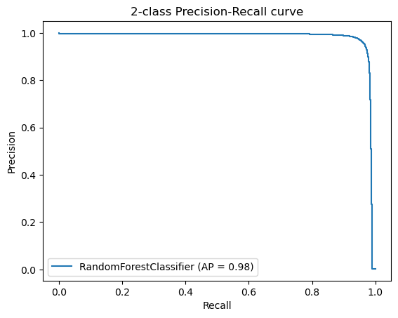
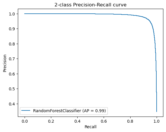
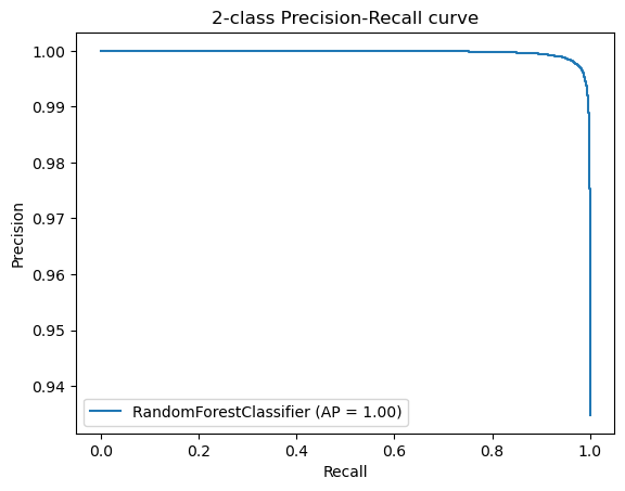
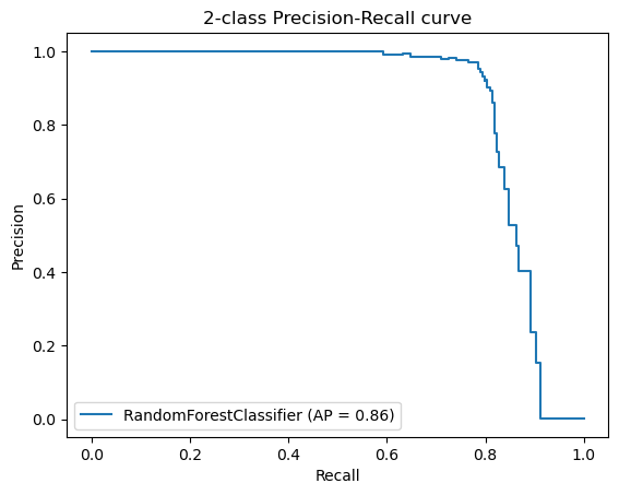
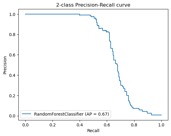
Additionally, we created Precision-Recall Curves on the same hold-out data. Precision-Recall curves are useful to determine the capability of the Model to predict the positive cases even in a highly unbalanced setting as we have for MutationTaster.